
Predictive Modeling - Regression Summary
1 Introduction
This blog post is a comprehensive summary of predictive modeling with regression techniques. It is Inspired by a lecture given by Sandjai Bhulai, Professor at the Free University of Amsterdam and co-founder of the postgraduate programme Business Analytics / Data Science. The main purpose is to have a quick look at the techniques and develop a proper workflow. The blog post also serves as my personal summary of the lecture.
2 Packages and initialisations
knitr::opts_chunk$set(echo = T, eval = T, warning = F, message = F, cache = T,
                      fig.align = "center", fig.width = 7, fig.height = 7)

## Load packages & Install if necessary
ipak <- function(pkg) {
  new.pkg <- pkg[!(pkg %in% installed.packages()[, "Package"])]
  if (length(new.pkg))
  install.packages(new.pkg, dependencies = TRUE)
  sapply(pkg, require, character.only = TRUE)
}


packages <- c("data.table", "ggthemes", "tidyverse", "DataExplorer", "kableExtra", "knitr", "data.table"
              ,"readr", "RColorBrewer", "htmlwidgets", "htmltools", "widgetframe", "highcharter", "elasticnet", "here")

ipak(packages)
## data.table ggthemes tidyverse DataExplorer kableExtra
## TRUE TRUE TRUE TRUE TRUE
## knitr data.table readr RColorBrewer htmlwidgets
## TRUE TRUE TRUE TRUE TRUE
## htmltools widgetframe highcharter elasticnet here
## TRUE TRUE TRUE TRUE TRUEtheme_set(theme_few()) # add few theme to plots3 Exploratory Data Analysis (EDA)
Quick look at the data.
FuelEff <- fread(here("static", "data","Regressions/FuelEfficiency.csv"))

FuelEff$ET <- as.factor(FuelEff$ET)
FuelEff$NC <- as.factor(FuelEff$NC)

glimpse(FuelEff)
## Observations: 38
## Variables: 8
## $ MPG <dbl> 16.9, 15.5, 19.2, 18.5, 30.0, 27.5, 27.2, 30.9, 20.3, 17.0...
## $ GPM <dbl> 5.917, 6.452, 5.208, 5.405, 3.333, 3.636, 3.676, 3.236, 4....
## $ WT <dbl> 4.360, 4.054, 3.605, 3.940, 2.155, 2.560, 2.300, 2.230, 2....
## $ DIS <int> 350, 351, 267, 360, 98, 134, 119, 105, 131, 163, 121, 163,...
## $ NC <fct> 8, 8, 8, 8, 4, 4, 4, 4, 5, 6, 4, 6, 6, 6, 6, 6, 8, 8, 8, 8...
## $ HP <int> 155, 142, 125, 150, 68, 95, 97, 75, 103, 125, 115, 133, 10...
## $ ACC <dbl> 14.9, 14.3, 15.0, 13.0, 16.5, 14.2, 14.7, 14.5, 15.9, 13.6...
## $ ET <fct> 1, 1, 1, 1, 0, 0, 0, 0, 0, 0, 0, 0, 0, 0, 0, 0, 1, 1, 1, 1...Below you will find a few descriptive plots of the data, which is important to have before you start with the actual predictions
3.1 Missing Values
There are no missing values
plot_missing(FuelEff)
3.2 Discrete Variables
plot_bar(FuelEff, title = "Bar charts of all discrete variables")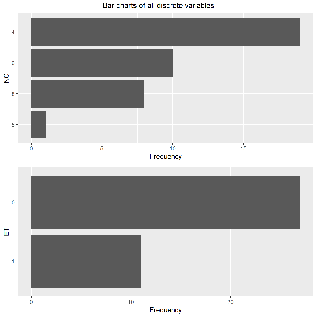
3.3 Continuous Variables
plot_histogram(FuelEff, title = "Histograms of all continues variables")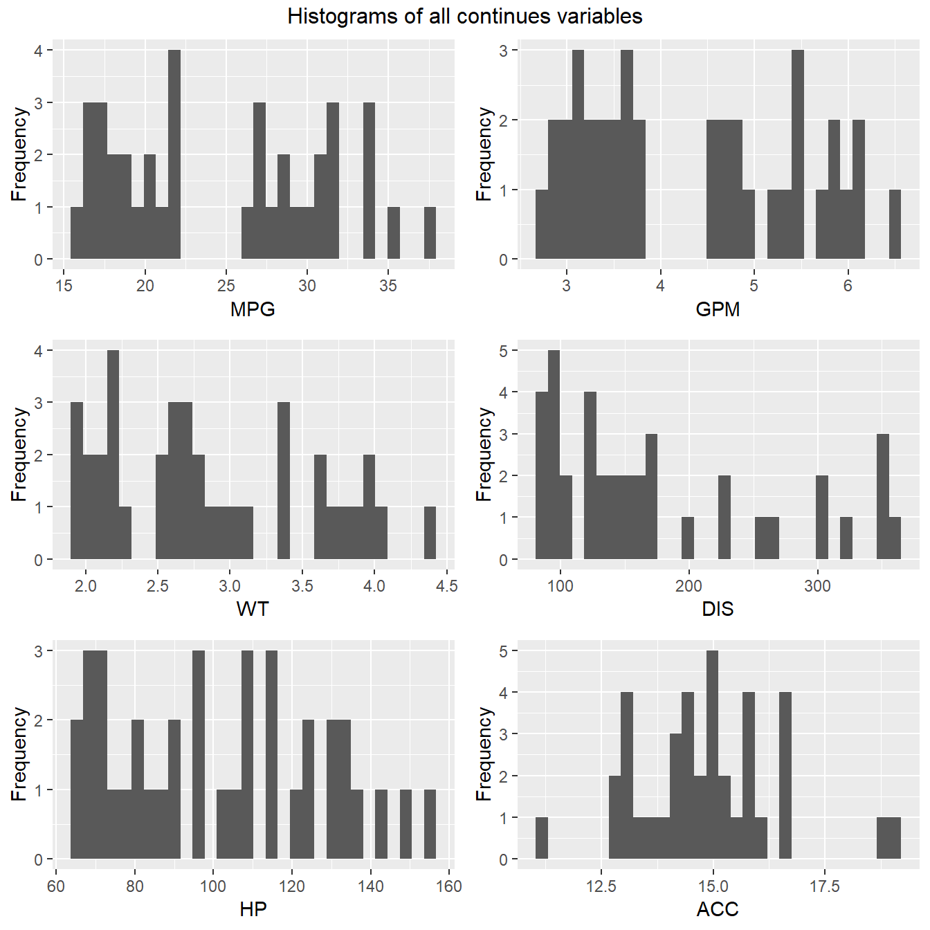
3.4 Correlations
plot_correlation(FuelEff, use = "pairwise.complete.obs", title = "Correlation Matrix")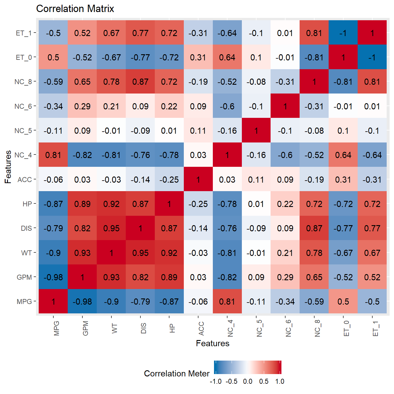
3.5 Boxplots
plot_boxplot(FuelEff, "MPG", title = "Boxplot of all variables with target variable MPG")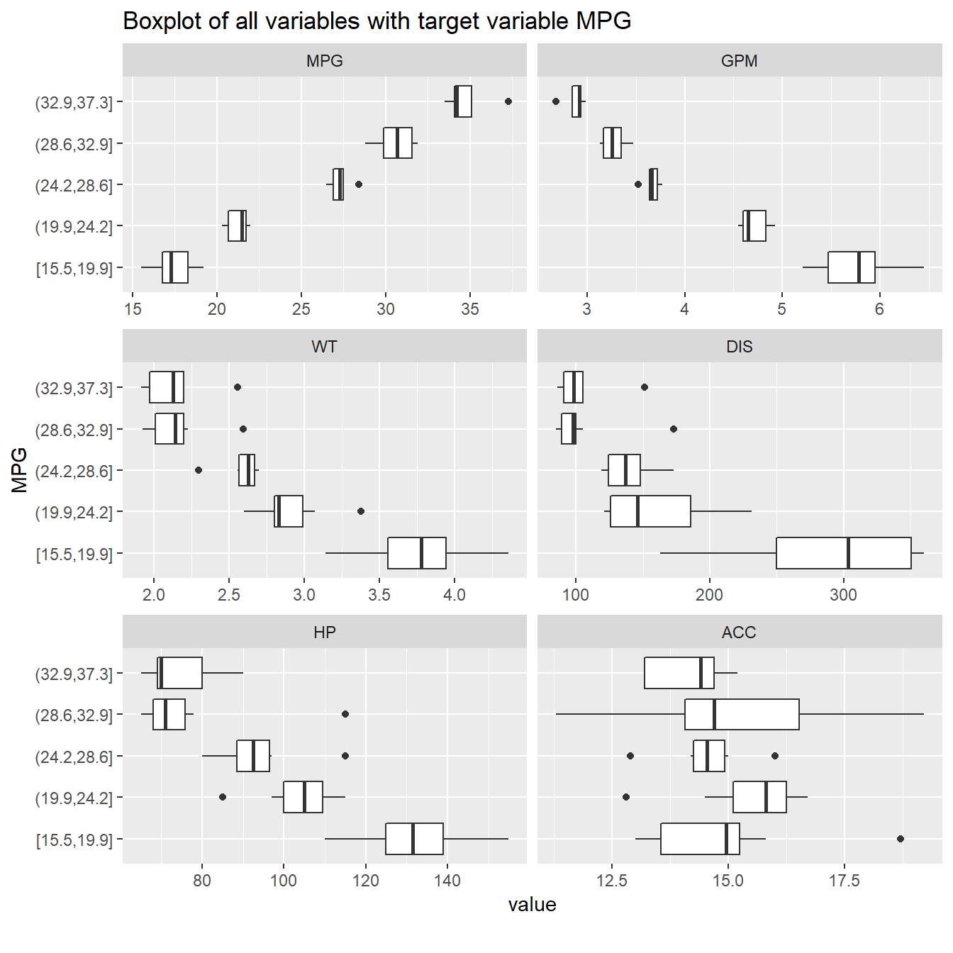
4 Data Description
Especially the correlation plots and box plots give a good indication of which variables might be important for your predictions. In this particular case, we see that WT, HP and DIS will likely be strong predictors, while ACC will not have a lot of impact. In larger datasets, there are many more steps to take before we select the eventual features.
5 Data Preparation
The current example dataset is small and easy to understand. However, it is good practice to perform a multitude of data preparation steps. The following steps are all useful and should always be considered before you start with machine learning.
- Centering & Scaling
- Check for skewness
- Rule of Thumb : (Largest / Smallest) > 20 = significant skewness
- Use BoxCox tests to transform predictors and remove the skewness
- Check for outliers
- Do not just throw away anything you think is an outlier. Think about the implications!
- Be careful with sampling your dataset - outliers might not be outliers at all.
- Check with experts about the collected data, they might know the reason for outliers.
- Data reduction & feature extraction
- Not a big issue in small datasets. But for large datasets, it will massively increase performance, and often have better results too.
- PCA is a great technique to use.
- Dealing with missing values
- Check for structurally missign values (might be mistakes in data collection, or surveys)
- Missing data might be informative!
- Data might be censored
- Imputate missing values. Choose appropriate methods.
- Using the data (mean, median)
- Random Draw
- Remove the samples
- Remove predictor (if large % missing)
- PCA to detect correlations
- KNN to fill in according to neighbouring values
- Removing predictors
- Remove predictors with near-zero variance
- Remove multicollinearity
- Adding predictors
- Higher-order predictors might increase performance
- Dummy variables for categorical data
- Binning variables
- Do not do this manually!
6 Model Choices
Choosing a model is not straightforward. There is a large variety of models, where each model excels at different things.
Generally speaking, the best practice is to start with several models that are the least interpretable and most flexible, such as
Boosted TreesorSupport Vector Machines (SVM). These models generally produce the most optimum results among a wide variety of predictions.It is then adviced to investigate simpler, less opaque, models, such as
Patial Least Squares (PLS),Generalized Additive Models (GAM)orMultivariate Addeptive Regression Splines (MARS).Use the simplest model that reasonably approximates the performance of the more complex methods - unless the complexity is not an issue (which is rarely the case).
See the image below for a quick summary of regression techniques.
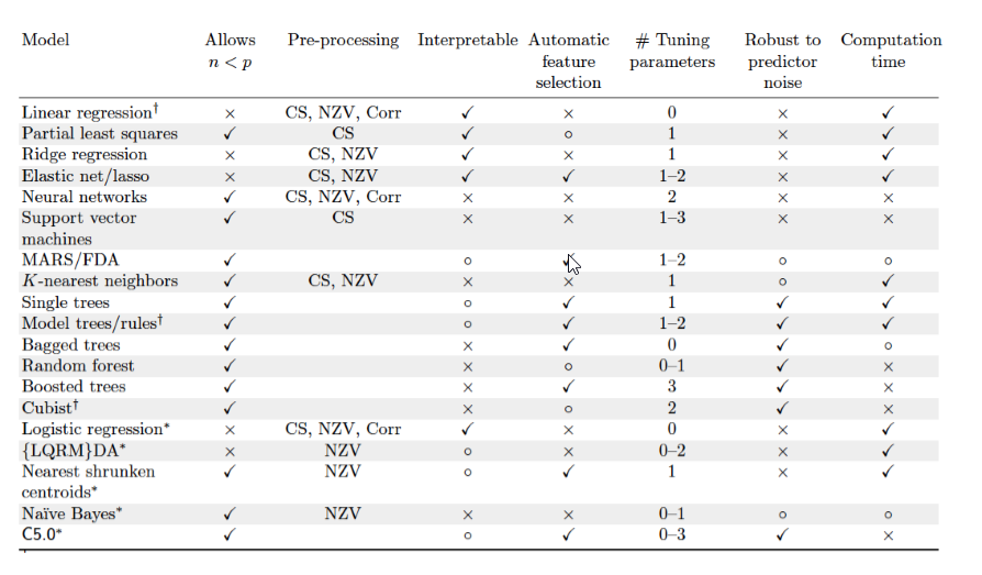
7 Model Preparations
Each model requires different parameters. Tuning these parameters is extremely important for your model performances. The image above shows the complexity of tuning the parameters (e.g. 0 is easy, 2 is hard) for each model. Wrong parameters can easily lead to bias, variance or overfitting of your model.
To reduce these issues, a variety of techniques for training your data can be used. The most common ones are Cross-Validation (CV) and Leave One Out Cross Validation (LOOCV).
In R, the easiest way to train models, and set control parameters is with the package Caret. Which is what I will be using as well.
library(caret)
FuelEff <- fread(here("static", "data", "Regressions/FuelEfficiency.csv"))
FuelEff <- FuelEff[, -1] %>%
  as.data.frame()

#ctrl <- trainControl(method = "LOOCV")
ctrl <- trainControl(method = "cv", number = 10)

traindata <- FuelEff[, 2:7]
response <- FuelEff[, 1]
8 Applying the Models
It is important to set the same seed for each model, so we can 1) compare the models on the same data, and 2) reproduce the same results.
8.1 Linear Regression
set.seed(123)
lmFit <- train(x = traindata,
               y = response,
               method = "lm",
               preProc = c("center", "scale"),
               trControl = ctrl)
lmFit
## Linear Regression
##
## 38 samples
## 6 predictor
##
## Pre-processing: centered (6), scaled (6)
## Resampling: Cross-Validated (10 fold)
## Summary of sample sizes: 34, 35, 35, 34, 34, 34, ...
## Resampling results:
##
## RMSE Rsquared MAE
## 0.3491038 0.9187413 0.2965739
##
## Tuning parameter 'intercept' was held constant at a value of TRUE8.2 Partial Least Squares
set.seed(123)
plsFit <-
  train(x = traindata,
        y = response,
        method = "pls",
        preProc = c("center", "scale"),
        trControl = ctrl)
plsFit
## Partial Least Squares
##
## 38 samples
## 6 predictor
##
## Pre-processing: centered (6), scaled (6)
## Resampling: Cross-Validated (10 fold)
## Summary of sample sizes: 34, 35, 35, 34, 34, 34, ...
## Resampling results across tuning parameters:
##
## ncomp RMSE Rsquared MAE
## 1 0.5342822 0.8222915 0.4320590
## 2 0.4340009 0.8679883 0.3488201
## 3 0.3860258 0.9311885 0.3216491
##
## RMSE was used to select the optimal model using the smallest value.
## The final value used for the model was ncomp = 3.plot(plsFit)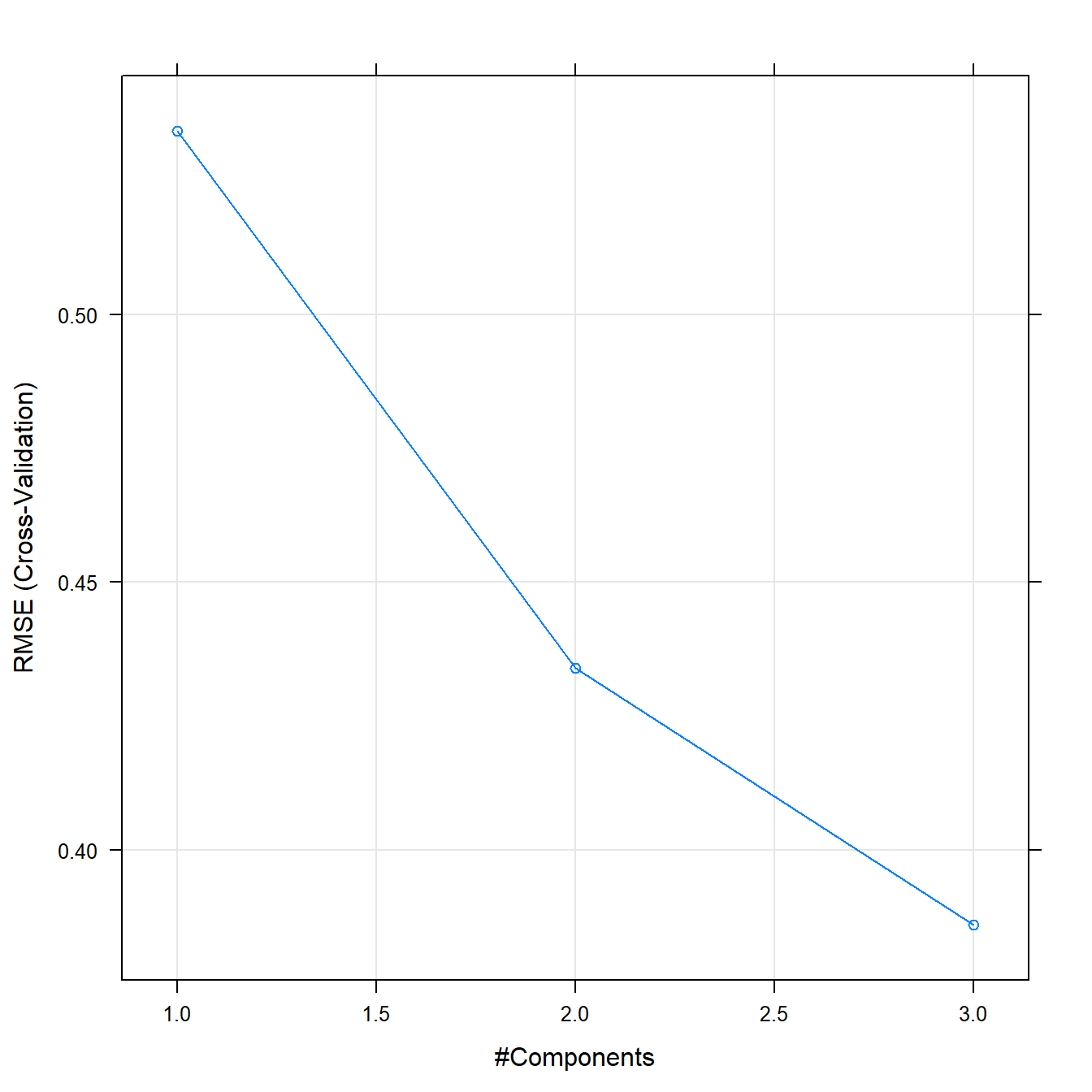
8.3 Principal Component Regression
set.seed(123)
pcrFit <-
  train(x = traindata,
        y = response,
        method = "pcr",
        preProc = c("center", "scale"),
        trControl = ctrl)
pcrFit
## Principal Component Analysis
##
## 38 samples
## 6 predictor
##
## Pre-processing: centered (6), scaled (6)
## Resampling: Cross-Validated (10 fold)
## Summary of sample sizes: 34, 35, 35, 34, 34, 34, ...
## Resampling results across tuning parameters:
##
## ncomp RMSE Rsquared MAE
## 1 0.5901381 0.8066295 0.4767139
## 2 0.5190486 0.8306519 0.4254869
## 3 0.4124337 0.9203584 0.3402541
##
## RMSE was used to select the optimal model using the smallest value.
## The final value used for the model was ncomp = 3.plot(pcrFit)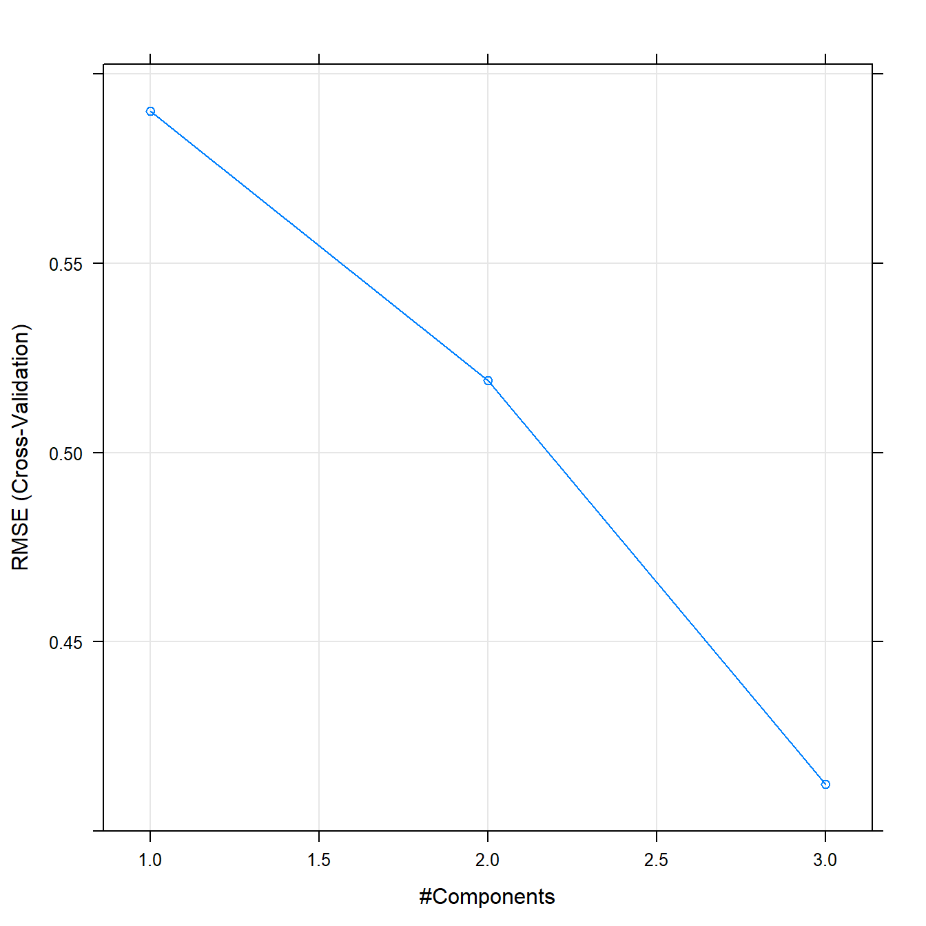
8.4 Ridge Regression
set.seed(123)
ridgeGrid <-
  data.frame(.lambda = seq(0, .1, length = 15)) #Lambda definitie

ridgeFit <-
  train(
    x = traindata,
    y = response,
    method = "ridge",
    preProc = c("center", "scale"),
    tuneGrid = ridgeGrid,
    trControl = ctrl
  )
ridgeFit
## Ridge Regression
##
## 38 samples
## 6 predictor
##
## Pre-processing: centered (6), scaled (6)
## Resampling: Cross-Validated (10 fold)
## Summary of sample sizes: 34, 35, 35, 34, 34, 34, ...
## Resampling results across tuning parameters:
##
## lambda RMSE Rsquared MAE
## 0.000000000 0.3491038 0.9187413 0.2965739
## 0.007142857 0.3491084 0.9202143 0.3001565
## 0.014285714 0.3507518 0.9207730 0.3028851
## 0.021428571 0.3529498 0.9206881 0.3051401
## 0.028571429 0.3552928 0.9201613 0.3070819
## 0.035714286 0.3576155 0.9193276 0.3088000
## 0.042857143 0.3598528 0.9182768 0.3103513
## 0.050000000 0.3619842 0.9170698 0.3117746
## 0.057142857 0.3640082 0.9157489 0.3130972
## 0.064285714 0.3659322 0.9143445 0.3143393
## 0.071428571 0.3677669 0.9128791 0.3155160
## 0.078571429 0.3695238 0.9113699 0.3166387
## 0.085714286 0.3712140 0.9098305 0.3179670
## 0.092857143 0.3728477 0.9082714 0.3196433
## 0.100000000 0.3744343 0.9067017 0.3212299
##
## RMSE was used to select the optimal model using the smallest value.
## The final value used for the model was lambda = 0.plot(ridgeFit)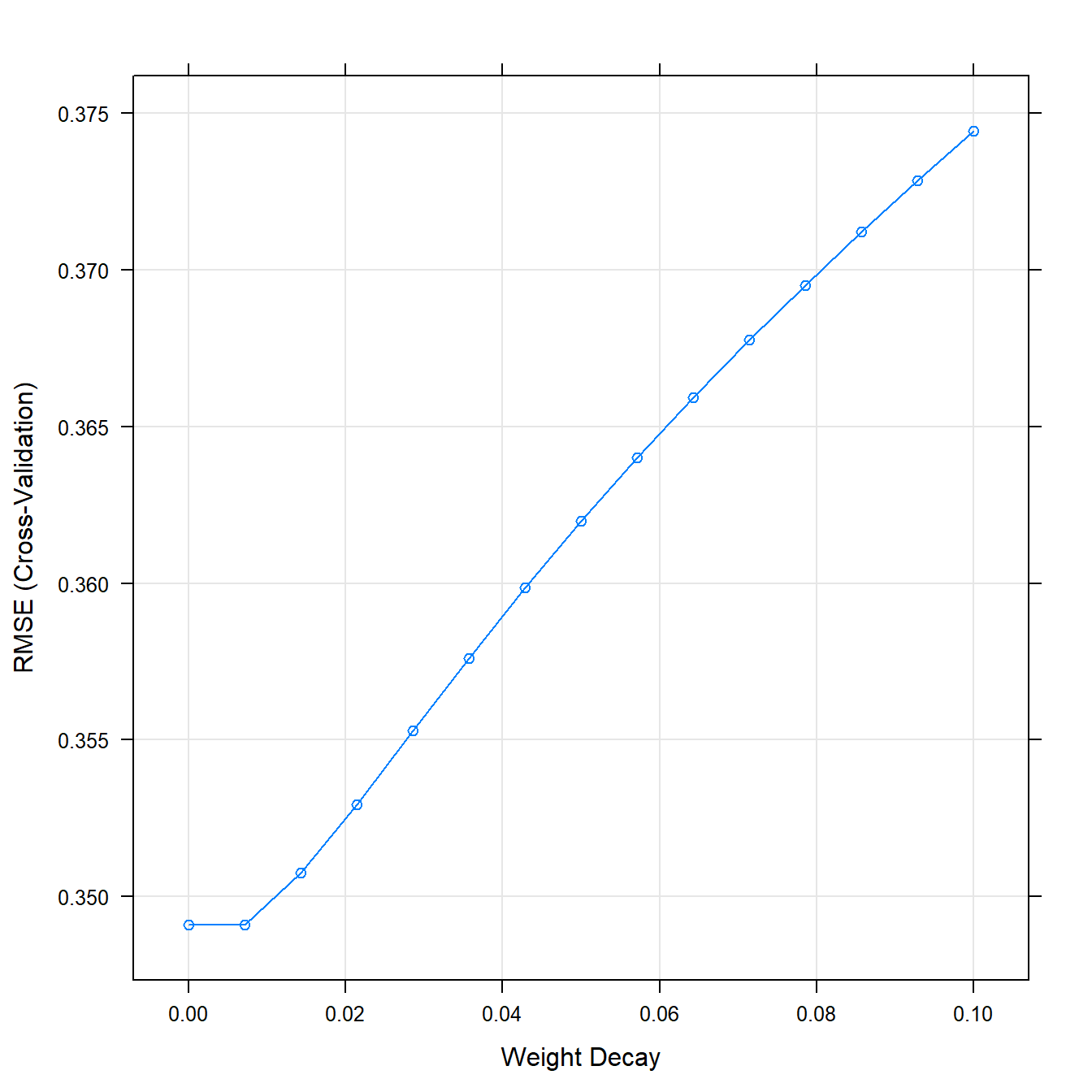
8.5 Lasso Regression
set.seed(123)
lassoGrid <- data.frame(.fraction = seq(0.05, 1, length = 20))
lassoFit <-
  train(
    x = traindata,
    y = response,
    method = "lars",
    preProc = c("center", "scale"),
    tuneGrid = lassoGrid,
    trControl = ctrl
  )
lassoFit
## Least Angle Regression
##
## 38 samples
## 6 predictor
##
## Pre-processing: centered (6), scaled (6)
## Resampling: Cross-Validated (10 fold)
## Summary of sample sizes: 34, 35, 35, 34, 34, 34, ...
## Resampling results across tuning parameters:
##
## fraction RMSE Rsquared MAE
## 0.05 0.9914435 0.8821032 0.9225322
## 0.10 0.8691388 0.8810176 0.8078626
## 0.15 0.7524983 0.8757677 0.6955019
## 0.20 0.6419761 0.8694007 0.5849300
## 0.25 0.5404261 0.8626244 0.4768875
## 0.30 0.4534510 0.8572930 0.3876725
## 0.35 0.4148866 0.8568022 0.3519432
## 0.40 0.4124938 0.8648776 0.3544209
## 0.45 0.4083596 0.8716531 0.3480199
## 0.50 0.3990464 0.8835669 0.3377982
## 0.55 0.3878828 0.8953990 0.3266916
## 0.60 0.3787880 0.9038286 0.3201525
## 0.65 0.3723993 0.9092132 0.3172129
## 0.70 0.3697524 0.9126979 0.3165587
## 0.75 0.3688900 0.9130463 0.3163729
## 0.80 0.3658178 0.9142300 0.3145681
## 0.85 0.3603385 0.9158821 0.3102977
## 0.90 0.3554954 0.9171826 0.3057231
## 0.95 0.3517300 0.9181306 0.3011485
## 1.00 0.3491038 0.9187413 0.2965739
##
## RMSE was used to select the optimal model using the smallest value.
## The final value used for the model was fraction = 1.plot(lassoFit)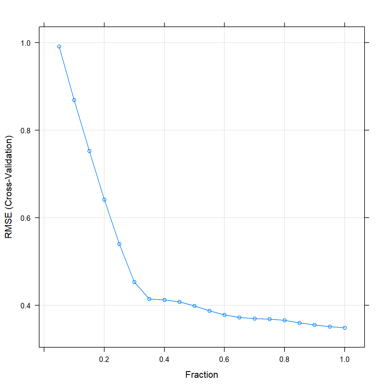
8.6 Elestic Net
set.seed(123)
enetGrid <-
  expand.grid(.lambda = c(0, 0.01, .1),
              .fraction = seq(.05, 1, length = 20))
enetFit <-
  train(
    x = traindata,
    y = response,
    method = "enet",
    preProc = c("center", "scale"),
    tuneGrid = enetGrid,
    trControl = ctrl
  )
enetFit
## Elasticnet
##
## 38 samples
## 6 predictor
##
## Pre-processing: centered (6), scaled (6)
## Resampling: Cross-Validated (10 fold)
## Summary of sample sizes: 34, 35, 35, 34, 34, 34, ...
## Resampling results across tuning parameters:
##
## lambda fraction RMSE Rsquared MAE
## 0.00 0.05 0.9914435 0.8821032 0.9225322
## 0.00 0.10 0.8691388 0.8810176 0.8078626
## 0.00 0.15 0.7524983 0.8757677 0.6955019
## 0.00 0.20 0.6419761 0.8694007 0.5849300
## 0.00 0.25 0.5404261 0.8626244 0.4768875
## 0.00 0.30 0.4534510 0.8572930 0.3876725
## 0.00 0.35 0.4148866 0.8568022 0.3519432
## 0.00 0.40 0.4124938 0.8648776 0.3544209
## 0.00 0.45 0.4083596 0.8716531 0.3480199
## 0.00 0.50 0.3990464 0.8835669 0.3377982
## 0.00 0.55 0.3878828 0.8953990 0.3266916
## 0.00 0.60 0.3787880 0.9038286 0.3201525
## 0.00 0.65 0.3723993 0.9092132 0.3172129
## 0.00 0.70 0.3697524 0.9126979 0.3165587
## 0.00 0.75 0.3688900 0.9130463 0.3163729
## 0.00 0.80 0.3658178 0.9142300 0.3145681
## 0.00 0.85 0.3603385 0.9158821 0.3102977
## 0.00 0.90 0.3554954 0.9171826 0.3057231
## 0.00 0.95 0.3517300 0.9181306 0.3011485
## 0.00 1.00 0.3491038 0.9187413 0.2965739
## 0.01 0.05 1.0021737 0.8821032 0.9324097
## 0.01 0.10 0.8901040 0.8809871 0.8275808
## 0.01 0.15 0.7826987 0.8755224 0.7249137
## 0.01 0.20 0.6800796 0.8690532 0.6238765
## 0.01 0.25 0.5838516 0.8619770 0.5250596
## 0.01 0.30 0.4958268 0.8564919 0.4316494
## 0.01 0.35 0.4352548 0.8531532 0.3672571
## 0.01 0.40 0.4194547 0.8543208 0.3586732
## 0.01 0.45 0.4155285 0.8571756 0.3554100
## 0.01 0.50 0.4102322 0.8658767 0.3483506
## 0.01 0.55 0.3993022 0.8799371 0.3382498
## 0.01 0.60 0.3885199 0.8924834 0.3283067
## 0.01 0.65 0.3796402 0.9021405 0.3202953
## 0.01 0.70 0.3733477 0.9089035 0.3171051
## 0.01 0.75 0.3690766 0.9142236 0.3137839
## 0.01 0.80 0.3674409 0.9153729 0.3138569
## 0.01 0.85 0.3629853 0.9170631 0.3116112
## 0.01 0.90 0.3577906 0.9185066 0.3081810
## 0.01 0.95 0.3533306 0.9196578 0.3047508
## 0.01 1.00 0.3496541 0.9205312 0.3013206
## 0.10 0.05 1.0332806 0.8821032 0.9609821
## 0.10 0.10 0.9518415 0.8783502 0.8851119
## 0.10 0.15 0.8730545 0.8683000 0.8111682
## 0.10 0.20 0.7970407 0.8584787 0.7389782
## 0.10 0.25 0.7212938 0.8522060 0.6655895
## 0.10 0.30 0.6481007 0.8480263 0.5928386
## 0.10 0.35 0.5794113 0.8406220 0.5233410
## 0.10 0.40 0.5197609 0.8340106 0.4600211
## 0.10 0.45 0.4755120 0.8299935 0.4080893
## 0.10 0.50 0.4467121 0.8286540 0.3800511
## 0.10 0.55 0.4357717 0.8289656 0.3667490
## 0.10 0.60 0.4249146 0.8361190 0.3558767
## 0.10 0.65 0.4160983 0.8441368 0.3477751
## 0.10 0.70 0.4096045 0.8512172 0.3433161
## 0.10 0.75 0.3997441 0.8615736 0.3378336
## 0.10 0.80 0.3912180 0.8721311 0.3327923
## 0.10 0.85 0.3843666 0.8822711 0.3287078
## 0.10 0.90 0.3789450 0.8916914 0.3249573
## 0.10 0.95 0.3756573 0.8998559 0.3229113
## 0.10 1.00 0.3744343 0.9067017 0.3212299
##
## RMSE was used to select the optimal model using the smallest value.
## The final values used for the model were fraction = 1 and lambda = 0.plot(enetFit)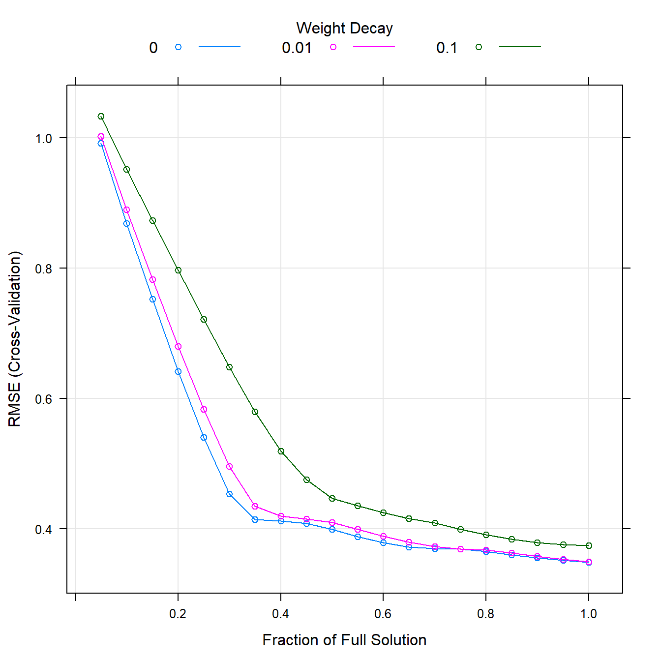
8.7 Neural Networks
Parameters
- Decay - sensitivity of the parameters. Used to balance overfitting / bias.
- Size - How many units the hidden layer has
- Bagging - Trying multiple neural networks and averaging these
- Linout - Linear output. Should be FALSE if doing classification instead of regression
- Trace - Shows everything that the model is doing - increases time
- maxNWts - Makes sure that you have enough memory to calculate the networks. If not - it won’t run.
- maxit - Maximum number of iterations before it stops, even if the network is not optimal yet.
set.seed(123)
nnetGrid <-
  expand.grid(.decay = c(0, 0.01, .1),
              .size = c(1:10),
              .bag = FALSE)
nnetFit <-
  train(
    traindata,
    response,
    method = "avNNet",
    tuneGrid = nnetGrid,
    trControl = ctrl,
    linout = TRUE,
    trace = FALSE,
    MaxNWts = 10 * (ncol(traindata) + 1) + 10 + 1,
    maxit = 500,
    preProc = c("center", "scale")
  )
nnetFit
## Model Averaged Neural Network
##
## 38 samples
## 6 predictor
##
## Pre-processing: centered (6), scaled (6)
## Resampling: Cross-Validated (10 fold)
## Summary of sample sizes: 34, 35, 35, 34, 34, 34, ...
## Resampling results across tuning parameters:
##
## decay size RMSE Rsquared MAE
## 0.00 1 0.3895405 0.8973923 0.3323903
## 0.00 2 0.6569133 0.8374466 0.5035775
## 0.00 3 0.6826297 0.8788383 0.5424810
## 0.00 4 0.8463658 0.6359670 0.6789124
## 0.00 5 0.7656605 0.7740208 0.6511560
## 0.00 6 0.8698821 0.7202164 0.7354869
## 0.00 7 1.0796775 0.6358712 0.8771279
## 0.00 8 1.0075220 0.6479410 0.8434621
## 0.00 9 0.8636968 0.7044664 0.7012957
## 0.00 10 0.9540263 0.6683322 0.7794921
## 0.01 1 0.3526006 0.9128624 0.3057678
## 0.01 2 0.3619619 0.9298032 0.3098504
## 0.01 3 0.3683206 0.9048323 0.3179104
## 0.01 4 0.3941588 0.9332994 0.3447662
## 0.01 5 0.4137627 0.9199535 0.3668975
## 0.01 6 0.4464267 0.8694082 0.3935072
## 0.01 7 0.4669006 0.8531353 0.4122863
## 0.01 8 0.4569140 0.8535870 0.4078636
## 0.01 9 0.4561972 0.8515777 0.4056808
## 0.01 10 0.4445728 0.8499994 0.3852996
## 0.10 1 0.3335752 0.9203501 0.2862332
## 0.10 2 0.3416498 0.9193257 0.2975506
## 0.10 3 0.3675403 0.9102944 0.3178251
## 0.10 4 0.3619042 0.9101573 0.3132779
## 0.10 5 0.3625173 0.9124789 0.3154598
## 0.10 6 0.3646521 0.9138108 0.3179842
## 0.10 7 0.3624660 0.9132400 0.3147886
## 0.10 8 0.3619679 0.9140112 0.3139177
## 0.10 9 0.3613569 0.9142954 0.3127367
## 0.10 10 0.3638330 0.9143804 0.3153601
##
## Tuning parameter 'bag' was held constant at a value of FALSE
## RMSE was used to select the optimal model using the smallest value.
## The final values used for the model were size = 1, decay = 0.1 and bag
## = FALSE.8.8 MARS
Parameters
- Pruning - Complexity degree of your model
set.seed(123)
marsGrid <- expand.grid(.degree = 1:2, .nprune = 2:38)
marsFit <-
  train(
    traindata,
    response,
    method = "earth",
    tuneGrid = marsGrid,
    trControl = ctrl
  )
marsFit
## Multivariate Adaptive Regression Spline
##
## 38 samples
## 6 predictor
##
## No pre-processing
## Resampling: Cross-Validated (10 fold)
## Summary of sample sizes: 34, 35, 35, 34, 34, 34, ...
## Resampling results across tuning parameters:
##
## degree nprune RMSE Rsquared MAE
## 1 2 0.4839472 0.8753910 0.4147103
## 1 3 0.5227159 0.8259529 0.4237267
## 1 4 0.4176467 0.8780799 0.3421071
## 1 5 0.4208958 0.8701870 0.3751769
## 1 6 0.4182763 0.8645150 0.3776940
## 1 7 0.4347006 0.8497555 0.3939607
## 1 8 0.4349547 0.8440440 0.3936475
## 1 9 0.4248572 0.8388525 0.3793411
## 1 10 0.4248572 0.8388525 0.3793411
## 1 11 0.4248572 0.8388525 0.3793411
## 1 12 0.4248572 0.8388525 0.3793411
## 1 13 0.4248572 0.8388525 0.3793411
## 1 14 0.4248572 0.8388525 0.3793411
## 1 15 0.4248572 0.8388525 0.3793411
## 1 16 0.4248572 0.8388525 0.3793411
## 1 17 0.4248572 0.8388525 0.3793411
## 1 18 0.4248572 0.8388525 0.3793411
## 1 19 0.4248572 0.8388525 0.3793411
## 1 20 0.4248572 0.8388525 0.3793411
## 1 21 0.4248572 0.8388525 0.3793411
## 1 22 0.4248572 0.8388525 0.3793411
## 1 23 0.4248572 0.8388525 0.3793411
## 1 24 0.4248572 0.8388525 0.3793411
## 1 25 0.4248572 0.8388525 0.3793411
## 1 26 0.4248572 0.8388525 0.3793411
## 1 27 0.4248572 0.8388525 0.3793411
## 1 28 0.4248572 0.8388525 0.3793411
## 1 29 0.4248572 0.8388525 0.3793411
## 1 30 0.4248572 0.8388525 0.3793411
## 1 31 0.4248572 0.8388525 0.3793411
## 1 32 0.4248572 0.8388525 0.3793411
## 1 33 0.4248572 0.8388525 0.3793411
## 1 34 0.4248572 0.8388525 0.3793411
## 1 35 0.4248572 0.8388525 0.3793411
## 1 36 0.4248572 0.8388525 0.3793411
## 1 37 0.4248572 0.8388525 0.3793411
## 1 38 0.4248572 0.8388525 0.3793411
## 2 2 0.4034104 0.8986415 0.3360562
## 2 3 0.4025746 0.8919200 0.3420545
## 2 4 0.3694814 0.8981198 0.3210576
## 2 5 0.3805058 0.8899355 0.3317454
## 2 6 0.3907333 0.8676445 0.3382646
## 2 7 0.3907333 0.8676445 0.3382646
## 2 8 0.3907333 0.8676445 0.3382646
## 2 9 0.3907333 0.8676445 0.3382646
## 2 10 0.3907333 0.8676445 0.3382646
## 2 11 0.3907333 0.8676445 0.3382646
## 2 12 0.3907333 0.8676445 0.3382646
## 2 13 0.3907333 0.8676445 0.3382646
## 2 14 0.3907333 0.8676445 0.3382646
## 2 15 0.3907333 0.8676445 0.3382646
## 2 16 0.3907333 0.8676445 0.3382646
## 2 17 0.3907333 0.8676445 0.3382646
## 2 18 0.3907333 0.8676445 0.3382646
## 2 19 0.3907333 0.8676445 0.3382646
## 2 20 0.3907333 0.8676445 0.3382646
## 2 21 0.3907333 0.8676445 0.3382646
## 2 22 0.3907333 0.8676445 0.3382646
## 2 23 0.3907333 0.8676445 0.3382646
## 2 24 0.3907333 0.8676445 0.3382646
## 2 25 0.3907333 0.8676445 0.3382646
## 2 26 0.3907333 0.8676445 0.3382646
## 2 27 0.3907333 0.8676445 0.3382646
## 2 28 0.3907333 0.8676445 0.3382646
## 2 29 0.3907333 0.8676445 0.3382646
## 2 30 0.3907333 0.8676445 0.3382646
## 2 31 0.3907333 0.8676445 0.3382646
## 2 32 0.3907333 0.8676445 0.3382646
## 2 33 0.3907333 0.8676445 0.3382646
## 2 34 0.3907333 0.8676445 0.3382646
## 2 35 0.3907333 0.8676445 0.3382646
## 2 36 0.3907333 0.8676445 0.3382646
## 2 37 0.3907333 0.8676445 0.3382646
## 2 38 0.3907333 0.8676445 0.3382646
##
## RMSE was used to select the optimal model using the smallest value.
## The final values used for the model were nprune = 4 and degree = 2.plot(marsFit)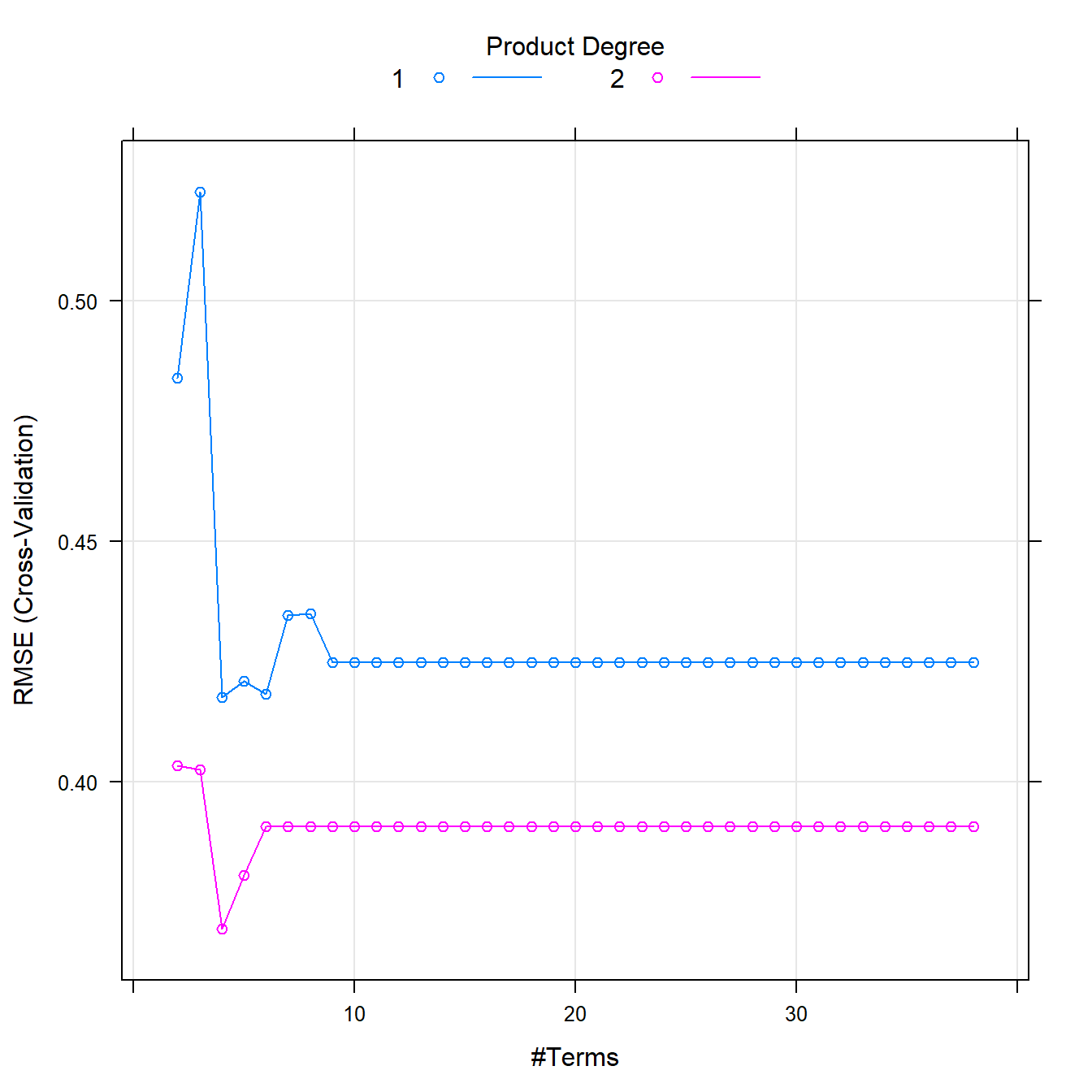
8.9 SVM
Parameters
- Can be either Radial / Polynomial / Linear
- Tunelength - Complexity
set.seed(123)
svmFit <-
  train(
    traindata,
    response,
    method = "svmRadial",
    tuneLength = 14,
    preProc = c("center", "scale"),
    trControl = ctrl
  )
svmFit
## Support Vector Machines with Radial Basis Function Kernel
##
## 38 samples
## 6 predictor
##
## Pre-processing: centered (6), scaled (6)
## Resampling: Cross-Validated (10 fold)
## Summary of sample sizes: 34, 35, 35, 34, 34, 34, ...
## Resampling results across tuning parameters:
##
## C RMSE Rsquared MAE
## 0.25 0.5919977 0.8378634 0.4865879
## 0.50 0.5236983 0.8676116 0.4471119
## 1.00 0.4691761 0.8957120 0.4029897
## 2.00 0.4564244 0.8537364 0.3931610
## 4.00 0.4563069 0.8448426 0.3945761
## 8.00 0.4660388 0.8455530 0.4041276
## 16.00 0.4733663 0.8418228 0.4093908
## 32.00 0.4728235 0.8409826 0.3994785
## 64.00 0.4903507 0.8238986 0.4114824
## 128.00 0.4907464 0.8235286 0.4118808
## 256.00 0.4907464 0.8235286 0.4118808
## 512.00 0.4907464 0.8235286 0.4118808
## 1024.00 0.4907464 0.8235286 0.4118808
## 2048.00 0.4907464 0.8235286 0.4118808
##
## Tuning parameter 'sigma' was held constant at a value of 0.4731597
## RMSE was used to select the optimal model using the smallest value.
## The final values used for the model were sigma = 0.4731597 and C = 4.plot(svmFit)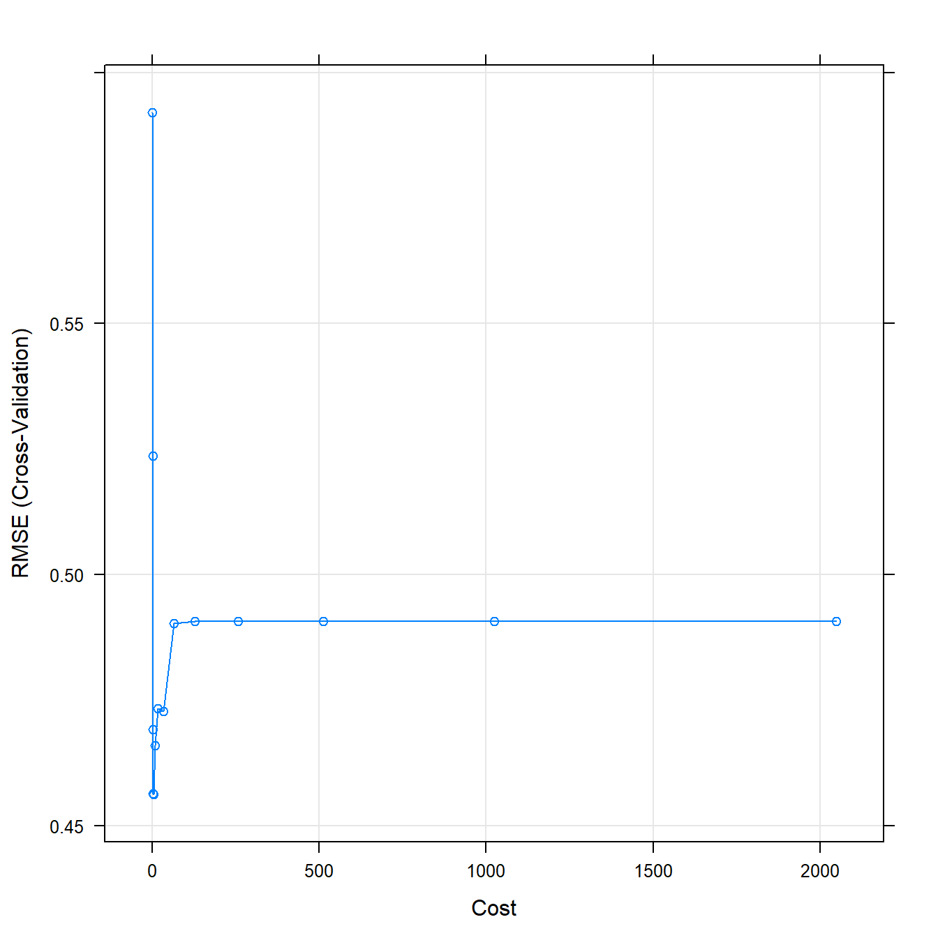
8.10 KNN
set.seed(123)
knnFit <-
  train(
    traindata,
    response,
    method = "knn",
    preProc = c("center", "scale"),
    tuneGrid = data.frame(.k = 1:20),
    trControl = ctrl
  )
knnFit
## k-Nearest Neighbors
##
## 38 samples
## 6 predictor
##
## Pre-processing: centered (6), scaled (6)
## Resampling: Cross-Validated (10 fold)
## Summary of sample sizes: 34, 35, 35, 34, 34, 34, ...
## Resampling results across tuning parameters:
##
## k RMSE Rsquared MAE
## 1 0.5414309 0.8170529 0.4652833
## 2 0.4698088 0.8428303 0.3928792
## 3 0.4989522 0.8224664 0.4212111
## 4 0.5056929 0.8219990 0.4109583
## 5 0.4905562 0.8513589 0.4127183
## 6 0.5027853 0.8368725 0.4288778
## 7 0.4926643 0.8435061 0.4278321
## 8 0.4883420 0.8315829 0.4261365
## 9 0.5170485 0.8297113 0.4485491
## 10 0.5324021 0.8230479 0.4611917
## 11 0.5519344 0.8178468 0.4777818
## 12 0.5572327 0.8253967 0.4820764
## 13 0.5587074 0.8345198 0.4788077
## 14 0.5869497 0.8309002 0.4998607
## 15 0.5949151 0.8369644 0.5142122
## 16 0.6090828 0.8410554 0.5257927
## 17 0.6261019 0.8322213 0.5506176
## 18 0.6560881 0.8039646 0.5795620
## 19 0.6904664 0.7902431 0.6047368
## 20 0.7291519 0.7881980 0.6467608
##
## RMSE was used to select the optimal model using the smallest value.
## The final value used for the model was k = 2.plot(knnFit)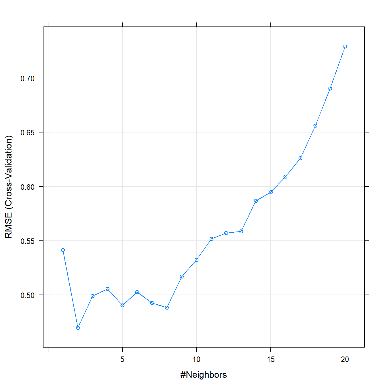
9 Model Performances
Evaluating performances of your model can be done by calculating a few statistical properties of the model and its predictions.
- Mean Absolute Error (MEA)
- Absolute difference between observed values and the model predictions
- Root Mean Squared Error (RMSE)
- Average distance between the observed values and the model predictions
- R²
- Proportion of information in the data that is explained by the model
- Is a correlation measure, not accuracy.
10 Model Comparison
allResamples <- resamples(
  list(
    "Linear Reg" = lmFit,
    "PLS" = plsFit,
    "PCR" = pcrFit,
    "Ridge" = ridgeFit,
    "LASSO" = lassoFit,
    "Elastic Net" = enetFit,
    "Neural Net" = nnetFit,
    "MARS" = marsFit,
    "SVM" = svmFit,
    "KNN" = knnFit
  )
)

gridExtra::grid.arrange(
parallelplot(allResamples, metric = "RMSE", main = "RMSE of each fold for each model"),
parallelplot(allResamples, metric = "Rsquared", main = "R² of each fold for each model"),
ncol = 2)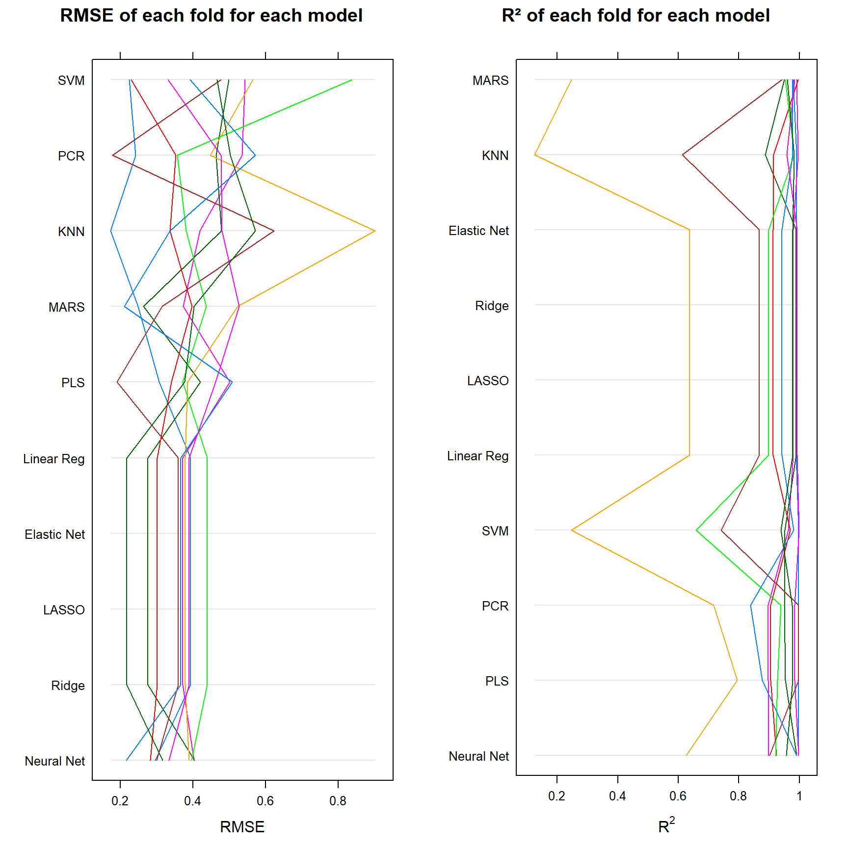
11 Final Notes
In the end, the final model that you choose to work with depends on a few factors. According to the summary, we should always choose a neural network in this particular example dataset. It is consistant throughout each fold, and gives very accurate predictions. However - it is harder to interpret and it takes up a lot more time than the other models.
For this reason, we might also select the next best things, i.e. Ridge Regression, Lasso, Elastic Net or even Linear Regression. These models are less consistent, yet still perform well, require a lot less time and are far easier to understand, explain and comprehend for every party (think clients, managers etc.) involved.
