
Introduction
I love traveling, and I love world maps, even more so when I can hang them on my walls. Now that got me thinking. What if I could create maps, with a similar look and feel, of all my holiday destinations? And what if I plot my location progression on top of the destination? That would be absolutely awesome!
In a recent post, I described how Google often tracks your location (if you agreed to it), and plotted each of my tracked location on a map. Now, I could easily subset that data on the time that I went on holiday, and plot that data on a map.
However, I noticed that after 2016, when I changed phones, I was no longer tracking my own GPS data.. (never thought I would be sad about a company not having tracked my complete whereabouts for over a year.) Anyway, I had to get creative and find a workaround. Now I knew that Google has a fantastic API, which solves all my problems!
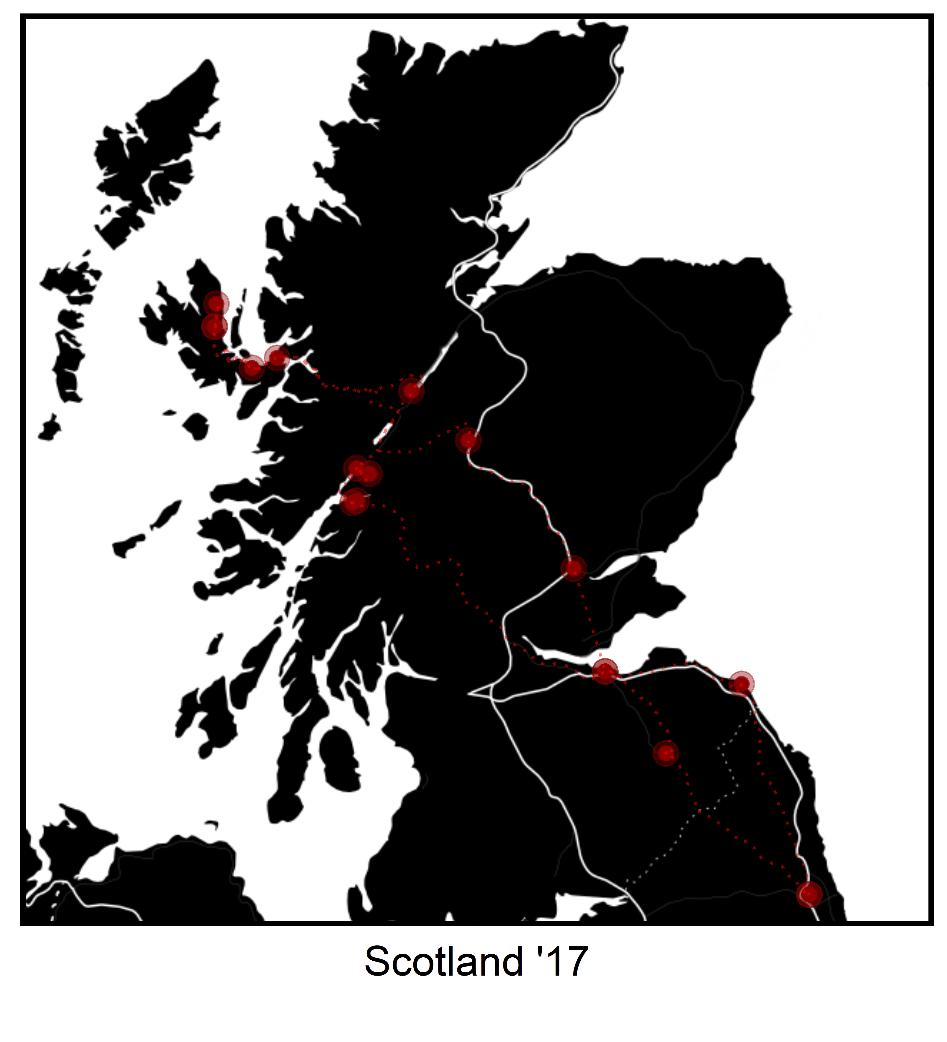
Let’s get started with my most recent holiday - Scotland - which is an absolutely stunning holiday destination. Especially around the Isle of Skye. The end product will look like this:
Background Map
## Load packages & Install if necessary
ipak <- function(pkg) {
  new.pkg <- pkg[!(pkg %in% installed.packages()[, "Package"])]
  if (length(new.pkg))
  install.packages(new.pkg, dependencies = TRUE)
  sapply(pkg, require, character.only = TRUE)
}


packages <- c("ggplot2", "ggmap", "ggthemes", "tidyverse")
ipak(packages)
## ggplot2 ggmap ggthemes tidyverse
## TRUE TRUE TRUE TRUEFirstly I had to find a background map which suited my style. In my opinion Stamen has the most beautiful maps with the Toner and Watercolor versions. Play around with the get_map options to find the right zoom level, maptype and color that you wish your background map to have. My setup gave me the following output:
toner_map <- get_map(c(-4.18265, 56.816922), #Insert the desired centre coordinates of your map
                     zoom = 7,
                     source='stamen',
                     maptype="toner-background",
                     color = "bw",
                     crop = TRUE)

ggmap(toner_map) +
  theme_map()
Now, I thought this background was a little too black, so I decided to create the inverse of the map.
## Inverted toner map
# invert colors in raster
invert <- function(x) rgb(t(255-col2rgb(x))/255)
toner_map_inv <- as.raster(apply(toner_map, 2, invert))

# copy attributes from original object
class(toner_map_inv) <- class(toner_map)
attr(toner_map_inv, "bb") <- attr(toner_map, "bb")

ggmap(toner_map_inv)+
  theme_map()
Looking sharp already! Now the next step is to plot my visited locations and trace my whereabouts step-wise.
Location Coordinates
- Step 1. Create a vector of the exact route with the full names, and often, the country.
- Google’s API sometimes gets confused when there are multiple cities with the same name. The API is not limited to cities. As you can see, I included **Old Man of Storr UK, which is a Point of Interest, and not a city, which also works!
# cities to geolocate
city_name <- c("Newcastle UK", "St. Abbs UK", "Edinburgh", "Ballachulish UK", "Glencoe UK", "Fort William UK","Ben Nevis UK", "Kyle of Lochalsh UK", "Broadford UK", "Portree UK" , "Old Man of Storr UK", "Portree UK", "Fort Augustus UK", "Dalwhinnie UK", "Perth UK", "Edinburgh", "Melrose UK", "Newcastle UK")

# initialize dataframe
 cities <- tibble(
  city = city_name,
  lon = rep(NA, length(city_name)),
  lat = rep(NA, length(city_name))
)- Step 2. Use the function
geocodeto loop over the vector, and find the coordinates for each location- I used a nested while loop because of the rate limit on Google’s API, ensuring that all locations were geolocated.
# loop cities through API to overcome API request limit
for(c in city_name){
  temp <- tibble(lon = NA)
  # geolocate until found
  while(is.na(temp$lon)) {
    temp <- geocode(c)
  }
  # write to dataframe
  cities[cities$city == c, -1] <- temp
}

head(cities, n = 3)
## # A tibble: 3 x 3
## city lon lat
## <chr> <dbl> <dbl>
## 1 Newcastle UK -1.62 55.0
## 2 St. Abbs UK -2.14 55.9
## 3 Edinburgh -3.19 56.0- Step 3. We need a data frame where each route is tracked from the initial point to the next. i.e. from Newcastle to St. Abbs, from St. Abbs to Edinburgh and so on. First
#
cities_trek <- cities %>%
  mutate(from = lag(city),
         to = city ) %>%
  select(from, to) %>%
  filter(from != "NA")

head(cities_trek, n = 3)
## # A tibble: 3 x 2
## from to
## <chr> <chr>
## 1 Newcastle UK St. Abbs UK
## 2 St. Abbs UK Edinburgh
## 3 Edinburgh Ballachulish UK- Step 4. For each
fromandtocombination, thetrek()function returns a bunch of coordinates based on the parameters mode, structure and output. If for example, you want to visualize a walking route, you can change the mode.
# create a dataframe of each route, store in a list
treklist <- list()
for (i in 1:nrow(cities_trek)){
  trek_df <- trek(from = cities_trek$from[i], to = cities_trek$to[i], structure = "route", mode = "driving", output = "simple")
  treklist[[i]] <- trek_df
}

# bind all rows of each dataframe in the list to a new dataframe.
tracks <- do.call(rbind, treklist)

head(tracks, n = 10)
## lat lon route
## 1 54.97831 -1.61804 A
## 2 54.97970 -1.61712 A
## 3 54.98077 -1.61681 A
## 4 54.98159 -1.61663 A
## 5 54.98166 -1.61665 A
## 6 54.98271 -1.62026 A
## 7 54.98283 -1.62019 A
## 8 54.98383 -1.62286 A
## 9 54.98615 -1.63059 A
## 10 54.98890 -1.63958 A- Step 5. Plotting time!
Creating your own beautiful poster!
- Use
geom_points()to add markers for your cities dataframe. Add colors, alpha values and size to your own style. I liked the red contrast. I added multiple to create some sort of signal. - Use
geom_path()for your tracks dataframe, again, give it your own spin!
scot_map <- ggmap(toner_map_inv) +
  geom_point(data=cities, aes(lon, lat),
             alpha = 1, color = "DarkRed", size = 2)+
  geom_point(data=cities, aes(lon, lat),
             alpha = 0.7, color = "DarkRed", size = 2.5)+
  geom_point(data=cities, aes(lon, lat),
             alpha = 0.4, color = "DarkRed", size = 4.5)+
  geom_path(data=tracks, aes(lon,lat), color="red",
            size=0.6, alpha = 0.5, linetype = "dotted" )+
  labs(caption = "Scotland '17")+
  guides(alpha = FALSE,
         size = FALSE)+
  scale_size_continuous(range = c(1,3))+
  theme_map()+
  theme(plot.caption = element_text(hjust=0.5, size=rel(1.5), vjust = -0.5),
        panel.border = element_rect(colour = "black", fill=NA, size=2))

scot_map
#Use the function below if you want to save the image.
#  ggsave(filename = "Images/scotland_map.png", plot = scot_map,
#         width = 6.7, height = 7, units = 'cm',
#         scale = 2, dpi = 600)
Now all that is left to do is, find a frame, print the image and put it on your wall!
Bonus! Can’t choose the background map? Neither could I.
Which is why I created the script below, where you can specify your map choices in a list, and see them all together! Or save them all together.
# Regular Toner
toner_map <- get_map(c(-4.18265, 56.816922),
                     zoom = 7,
                     source='stamen',
                     maptype="toner-background",
                     color = "bw", crop = TRUE)

## Inverted toner map

invert <- function(x) rgb(t(255-col2rgb(x))/255)
toner_map_inv <- as.raster(apply(toner_map, 2, invert))

# copy attributes from original object
class(toner_map_inv) <- class(toner_map)
attr(toner_map_inv, "bb") <- attr(toner_map, "bb")

#Terrain map
terrain_map <- get_map(c(-4.18265, 56.816922), zoom = 7,
                       source='stamen',
                       maptype="terrain",
                       color = "color",
                       crop = TRUE)

#Terrain map BG
terrain_map_bg <- get_map(c(-4.18265, 56.816922),
                        zoom = 7,
                       source='stamen',
                       maptype="terrain-background",
                       color = "color", crop = TRUE)

#watercolor
watercolor <- get_map(c(-4.18265, 56.816922),
                        zoom = 7,
                       source='stamen',
                       maptype="watercolor",
                       color = "color", crop = TRUE)

#inverted watercolor
invert <- function(x) rgb(t(255-col2rgb(x))/255)
watercolor_inverted <- as.raster(apply(watercolor, 2, invert))

# copy attributes from original object
class(watercolor_inverted) <- class(watercolor)
attr(watercolor_inverted, "bb") <- attr(watercolor, "bb")

#List of all the maps
maplist <- list(terrain_map, terrain_map_bg, toner_map, toner_map_inv, watercolor, watercolor_inverted)
names(maplist)  <- c("terrain_map", "terrain_bg", "toner", "toner_inv", "watercolor", "watercolor_inverted")


#For loop
p <- list()
for (i in 1: length(maplist)){
 p[[i]] <-  ggmap(maplist[[i]]) +
  geom_point(data=cities, aes(lon, lat), alpha = 1, color = "DarkRed", size = 2)+
  geom_point(data=cities, aes(lon, lat), alpha = 0.7, color = "DarkRed", size = 2.5)+
  geom_point(data=cities, aes(lon, lat), alpha = 0.4, color = "DarkRed", size = 4.5)+
  geom_path(data=tracks, aes(lon,lat), color="red", size=0.6, alpha = 0.5, linetype = "dotted" )+
  labs(caption = "Scotland '17")+
  guides(alpha = FALSE,
         size = FALSE)+
  scale_size_continuous(range = c(1,3))+
  ggtitle(paste(names(maplist)[i]))+
  theme_map()+
  theme(plot.caption = element_text(hjust=0.5, size=rel(1.5), vjust = -0.5),
        plot.title = element_text(hjust = 0.5),
        panel.border = element_rect(colour = "black", fill=NA, size=2))
  }

gridExtra::grid.arrange(
  p[[1]], p[[2]], p[[3]], p[[4]], p[[5]], p[[6]], ncol = 2
)
Final thoughts
Hot damn that inverted Watercolor is actually really cool! Perhaps I’ll use that on my wall. I would love to see your renditions, so feel free to leave a comment here or send me an e-mail with your own creations!
